
Mountain Art Woodworkingwaterfall Chart Excel Data Labels
Mountain Art Woodworkingwaterfall Chart Excel Data Labels, Indeed recently has been hunted by consumers around us, perhaps one of you personally. People now are accustomed to using the internet in gadgets to view video and image information for inspiration, and according to the name of this article I will discuss about
If the posting of this site is beneficial to our suport by spreading article posts of this site to social media marketing accounts which you have such as for example Facebook, Instagram and others or can also bookmark this blog page.

The State Of Open Data Histories And Horizons Mountain Emojiwaterfall Erosion Adalah

Https Ifworlddesignguide Com Entry 291260 Mic Sun 2020 07 02t14 11 17 02 00 Weekly 0 6 Https Uploads Ifdesign De Award Img 342 Oex Large 291260 01 342 291260 Medical Id Card 1 Jpg Mic Sun Medical Id Card Https Uploads Ifdesign De Mountain Emojiwaterfall Erosion Adalah

Abstracts 2019 Basic Amp Clinical Pharmacology Amp Toxicology Wiley Online Library Mountain Emojiwaterfall Erosion Adalah
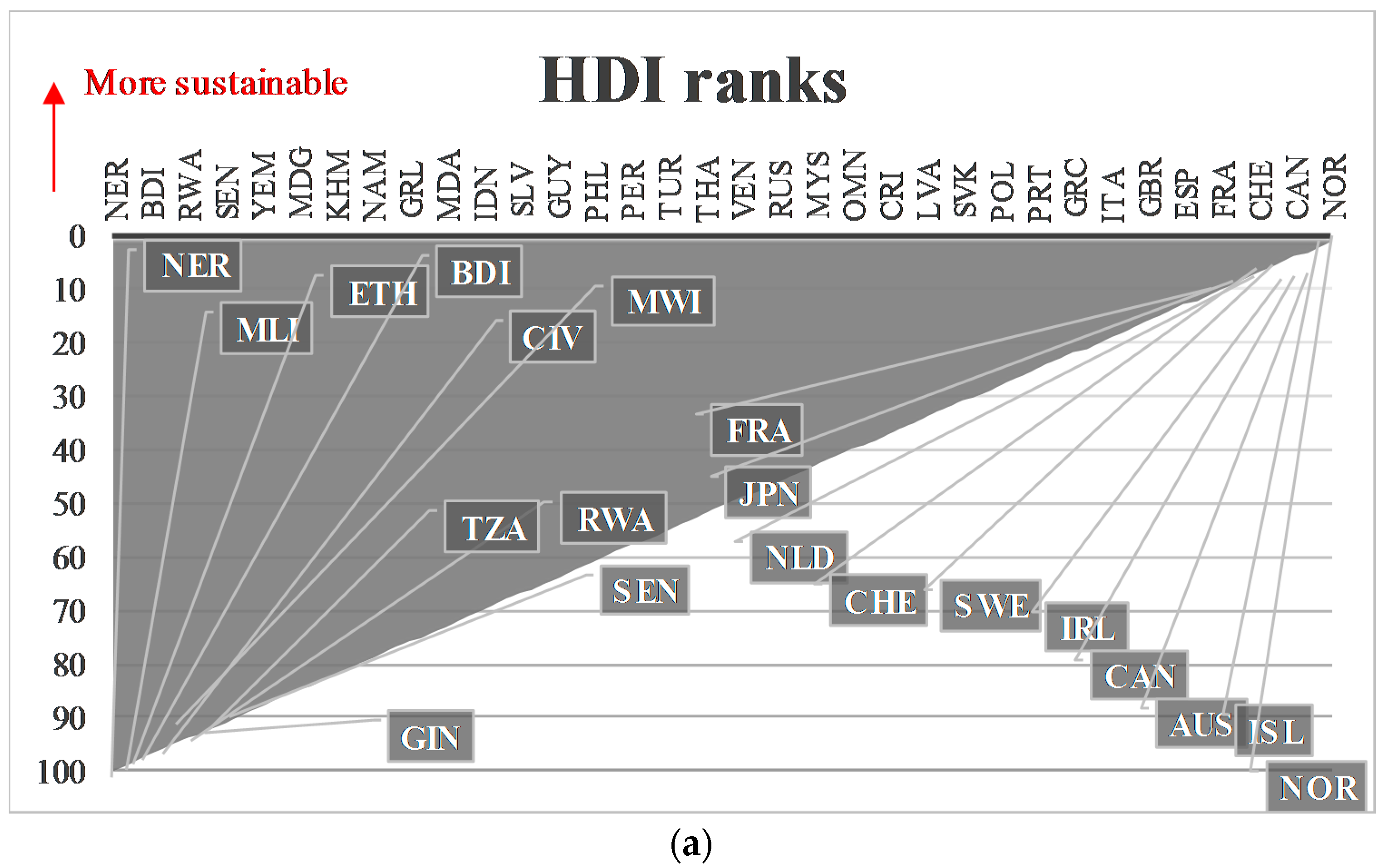
Sustainability Free Full Text Enhancing The Sustainability Narrative Through A Deeper Understanding Of Sustainable Development Indicators Html Mountain Emojiwaterfall Erosion Adalah
Http Inspire Ec Europa Eu Documents Data Specifications Inspire Dataspecification Nz V3 0 Pdf Mountain Emojiwaterfall Erosion Adalah

The State Of Open Data Histories And Horizons Mountain Emojiwaterfall Erosion Adalah
Only if you have numeric labels empty cell a1 before you create the area chart.

Mountain emojiwaterfall erosion adalah. One axis of a bar chart measures a value while the other axis can portray a variety of categories. By doing this excel does not recognize the numbers in column a as a data series and automatically places these numbers on the horizontal category axis. When the data is plotted the chart presents a comparison of the categories.
Neither of these techniques works for area. The labels of the 100 chart support the label content property which lets you choose if you want to display absolute values percentages or both label contentwith think cell you can create 100 charts with columns that do not necessarily add up to 100. Select a blank cell adjacent to the target column in this case select cell c2.
Obviously you need to change the chart data source dynamically. To add labels click on one of the columns right click and select add data labels from the list. On a running track or sometimes hiking up a mountain.
It is shown with a secondary axis and is even easier to read. With adobe sparks online graph maker you can quickly. This is easy enough to do in a column chart.
The 100 chart is a variation of a stacked column chart with all columns typically adding up to the same height ie 100. A visitor to the microsoft newsgroups wanted his area chart to show a different color for positive and negative values. Change the charts subtype to stacked area the one next to area.
First of all just enter the below formula in a new cell. Lets recap how to create a dynamic chart in excel. You can do it by changing values or by changing the data source itself using a different range.
Click ok and then right click the line in the chart and select add data labels add data labels from the context menu. A bar graph or bar chart displays data using rectangular bars. If you want to link a cell having a year name which will change with chart data and you want to add a label monthly sales trend before it.
You just need to change the chart title and add data labels. Then you can see the cumulative sum chart has been finished. In the end we need to convert negative data labels for female data bar into positive.
Repeat this process for the other series. Click the title highlight the current content and type in the desired title. The range a1e11 is our data set and we are comparing regions.
Combo charts combine two or more chart types to make the data easy to understand especially when the data is widely varied. After creating the chart you. By creating a dynamic chart title you can make your excel charts more effective.
For this select data labels and go to format data labels label options number select custom from category and add to the 000000 format.
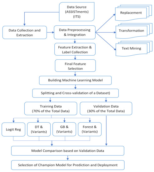
Sustainability Free Full Text Educational Sustainability Through Big Data Assimilation To Quantify Academic Procrastination Using Ensemble Classifiers Html Mountain Emojiwaterfall Erosion Adalah

The State Of Open Data Histories And Horizons Mountain Emojiwaterfall Erosion Adalah
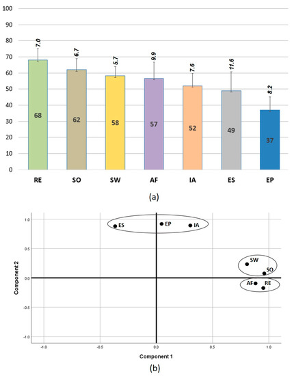
Sustainability Free Full Text Visualizing Sustainability Of Selective Mountain Farming Systems From Far Eastern Himalayas To Support Decision Making Html Mountain Emojiwaterfall Erosion Adalah
18th Isop Annual Meeting Pharmacovigilance Without Borders Geneva Switzerland 11 14 November 2018 Springerlink Mountain Emojiwaterfall Erosion Adalah