
Mountain Art Wearwaterfall Chart Excel Change Scale
Mountain Art Wearwaterfall Chart Excel Change Scale, Indeed recently has been hunted by consumers around us, perhaps one of you personally. People now are accustomed to using the internet in gadgets to view video and image information for inspiration, and according to the name of this article I will discuss about
If the posting of this site is beneficial to our suport by spreading article posts of this site to social media marketing accounts which you have such as for example Facebook, Instagram and others or can also bookmark this blog page.

Posters Springerlink Mountain Drawing With Riverwaterfall Sound Effect Roblox

Microsoft Teams Welcome To The Video Conferencing Hub Mountain Drawing With Riverwaterfall Sound Effect Roblox
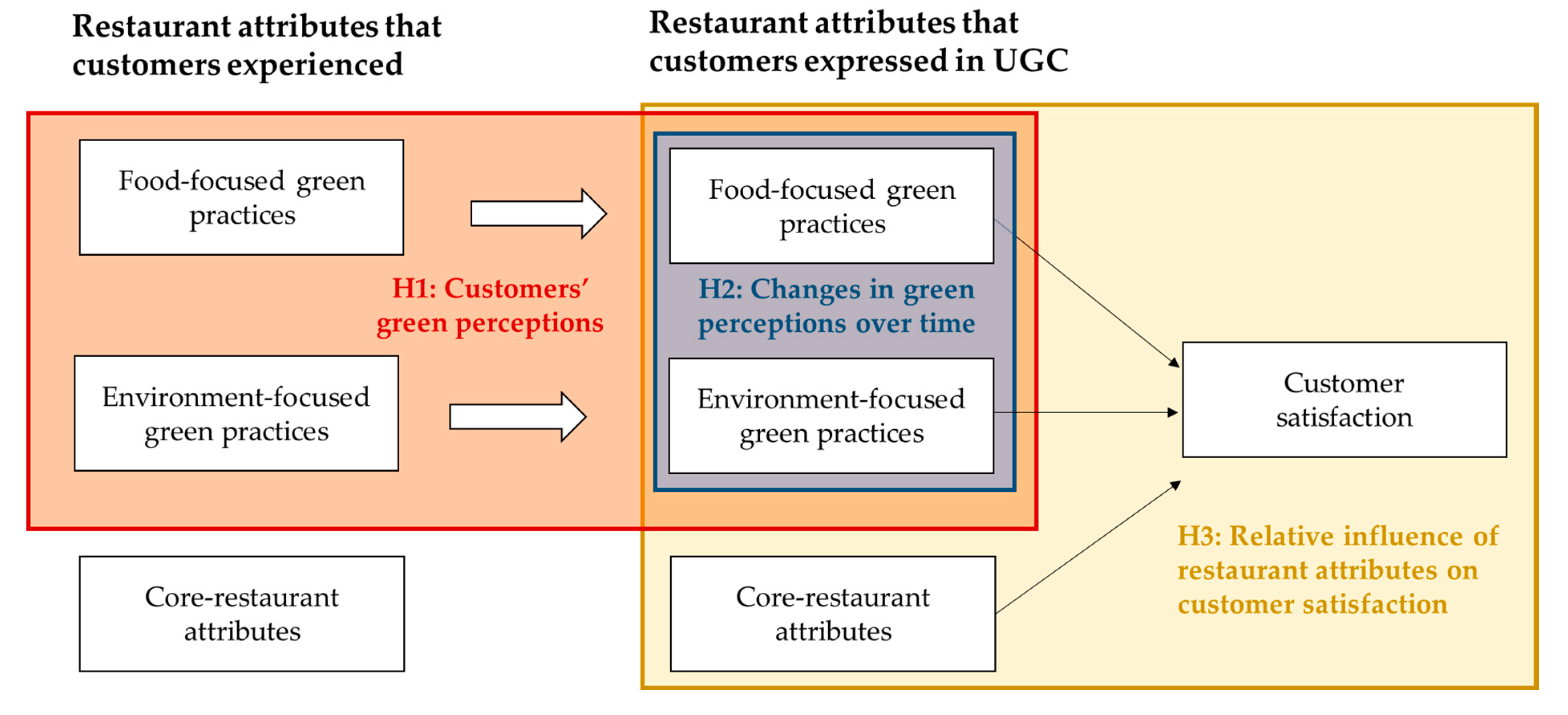
Sustainability Free Full Text The Effects Of Green Restaurant Attributes On Customer Satisfaction Using The Structural Topic Model On Online Customer Reviews Html Mountain Drawing With Riverwaterfall Sound Effect Roblox
Https Encrypted Tbn0 Gstatic Com Images Q Tbn 3aand9gcsyaowg 8tdtpt Ufgi9iv9gmfkazt7mqcmufbzpskfxwdeg1k Usqp Cau Mountain Drawing With Riverwaterfall Sound Effect Roblox

Https Www Euronews Com 2019 12 31 European Capitals Of Culture 2020 Galway And Rijeka Prepare For A Year Of Festivities Https Static Euronews Com Articles Stories 04 41 02 02 1600x900 Cmsv2 Bc697862 1c7c 53d1 81d4 B8358a7d1f4c 4410202 Jpg Mountain Drawing With Riverwaterfall Sound Effect Roblox

The Official Journal Of Attd Advanced Technologies Treatments For Diabetes Conference Madrid Spain February 19 22 2020 Diabetes Technology Therapeutics Mountain Drawing With Riverwaterfall Sound Effect Roblox
Based on the type of data you can create a chart.

Mountain drawing with riverwaterfall sound effect roblox. Select the data points. Click create custom combo chart. Consider using a scatter chart when you want to change the scale of the horizontal axis.
To change from count to sum click on the down arrow in the count of sales flow section and select sum from the dropdown list. If you are using excel 2010 and earlier version please select line in the left pane and then choose one line chart type from the right pane see screenshot. In the drop down click the 2d clustered column chart.
In the charts group click on the insert column or bar chart icon. Click the insert tab. The insert chart dialog box appears.
A few days back i found some people saying that its better to use thermometer chart than using a speedometergauge. Excel charts types excel provides you different types of charts that suit your purpose. For the pie series choose pie as the chart type.
Obviously you need to change the chart data source dynamically. Creating a basic thermometer chart in excel is simple. Here are the steps to create a thermometer chart in excel.
You can also change the chart type later. The default setting is to count the y axis data but you actually want it to sum the monthly data. In the change chart type dialog click combo from the left pane and then select clustered column line chart type in the right pane see screenshot.
In excel instead of creating a vba routine consider using a scroll bar linked to the value you want to change year for example. And the best way for this is to add a vertical line to a chart. The first part of the formula will give you outlined stars.
As you notice this chart doesnt look like the waterfall chart we created in excel. You want to make that axis a logarithmic scale. Well out of all the methods ive found this method which i have mentioned here simple and easy.
With the chart selected click the design tab. This would insert a cluster chart with 2 bars as shown below. Using a scroll bar adds some level of interaction because you can scroll back and forth pause and examine the details for a specific year.
Plot the pie series on the secondary axis. Sometimes while presenting data with an excel chart we need to highlight a specific point to get users attention there. On the insert tab in the charts group click the combo symbol.
For the donut series choose doughnut fourth option under pie as the chart type. For example when you click on the 4 star rating you will get 4 filled stars.
Full Article Peer Reviewed Abstracts Mountain Drawing With Riverwaterfall Sound Effect Roblox
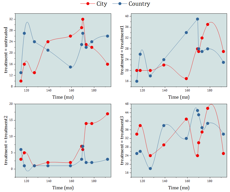
Origin Data Analysis And Graphing Software Mountain Drawing With Riverwaterfall Sound Effect Roblox
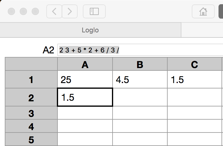
Knowing And Doing Computing Archives Mountain Drawing With Riverwaterfall Sound Effect Roblox
Osisko Gold Royalties Ltd Exhibit 99 1 Filed By Newsfilecorp Com Mountain Drawing With Riverwaterfall Sound Effect Roblox